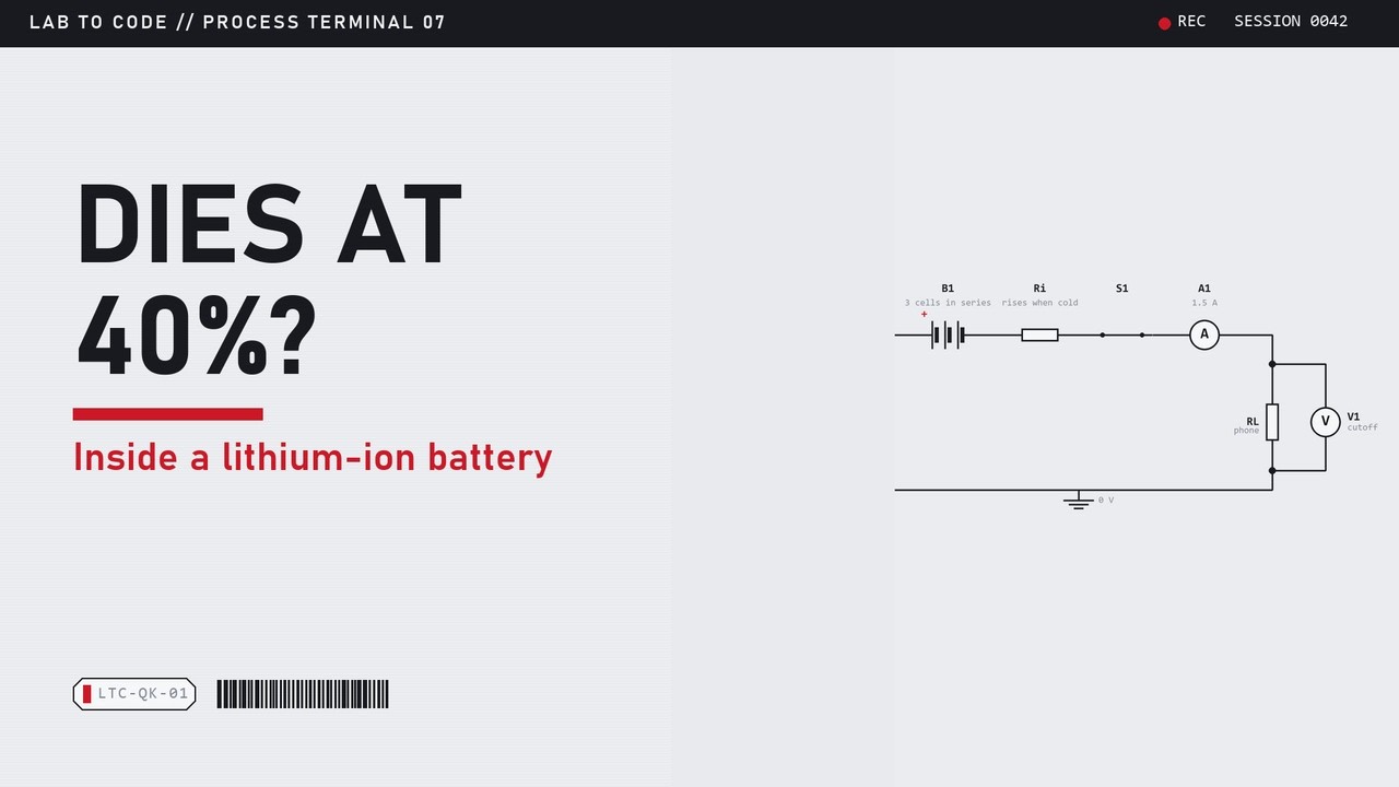
Why Your Phone Dies in the Cold: Inside a Lithium-Ion Battery
MODULE 01 // LTC
Química y datos, explicados simple (+ Python)Chemistry and data, explained simply (+ Python)
Cada video toma un concepto de química o de calidad de procesos, lo explica con un ejemplo real y termina con unas pocas líneas de Python que hacen el cálculo por ti. El código de cada sesión, ejecutado y con su salida real, está más abajo en esta página.Each video takes one chemistry or process-quality concept, explains it with a real example and ends with a few lines of Python that do the calculation for you. The code for every session, run and with its real output, is further down this page.







CODEDESCARGAR .PYDOWNLOAD .PY · VER EL VIDEOWATCH THE VIDEO →
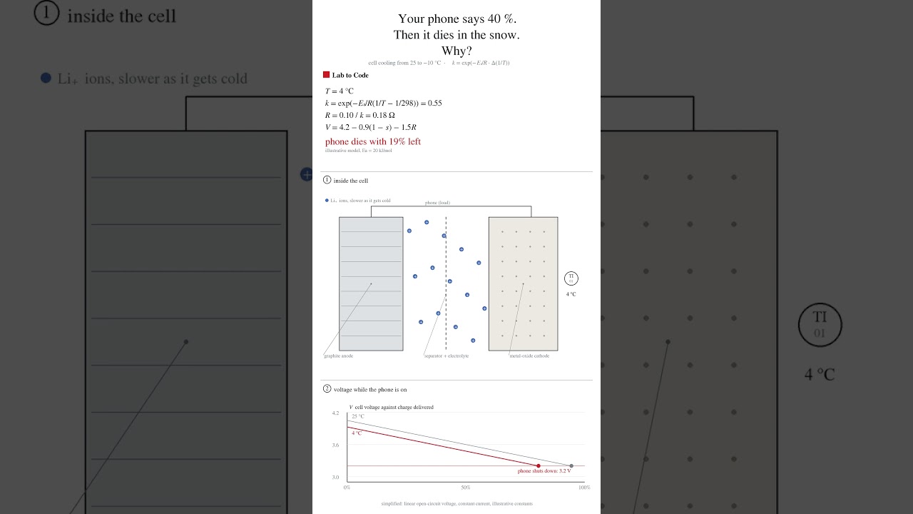
"""Lab to Code - Why a phone dies in the cold: Arrhenius ionic conductivity and internal resistance.

Model (illustrative parameters): the electrolyte's ionic conductivity follows Arrhenius with Ea = 20 kJ/mol,
so the cell's internal resistance grows as 1 / k when it cools. The phone draws I amps and shuts down when the
cell voltage, V = V_FULL - SPAN * (1 - s) - I * R, falls to V_CUT. Open-circuit voltage is taken as linear.
"""
from math import exp

R, EA, T0 = 8.314, 20e3, 298.15
V_FULL, V_CUT, SPAN = 4.2, 3.2, 0.9      # volts: full charge, phone shutdown, open-circuit span
R25, I = 0.10, 1.5                        # ohm at 25 C, amps drawn by the phone

for t_c in (25, 10, 0, -10, -20):
    k = exp(-EA / R * (1 / (t_c + 273.15) - 1 / T0))      # conductivity relative to 25 C
    r = R25 / k
    usable = min(1.0, max(0.0, (V_FULL - V_CUT - I * r) / SPAN))
    print(f"{t_c:3} C: k = {k:4.2f}, resistance {r:5.2f} ohm, phone dies with {1 - usable:4.0%} left")
SALIDA REALREAL OUTPUT
 25 C: k = 1.00, resistance  0.10 ohm, phone dies with   6% left
 10 C: k = 0.65, resistance  0.15 ohm, phone dies with  14% left
  0 C: k = 0.48, resistance  0.21 ohm, phone dies with  24% left
-10 C: k = 0.34, resistance  0.29 ohm, phone dies with  38% left
-20 C: k = 0.24, resistance 0.42 ohm, phone dies with 59% leftCODEDESCARGAR .PYDOWNLOAD .PY · VER EL VIDEOWATCH THE VIDEO →
"""Lab to Code - Why a phone dies in the cold: Arrhenius ionic conductivity and internal resistance.

Model (illustrative parameters): the electrolyte's ionic conductivity follows Arrhenius with Ea = 20 kJ/mol,
so the cell's internal resistance grows as 1 / k when it cools. The phone draws I amps and shuts down when the
cell voltage, V = V_FULL - SPAN * (1 - s) - I * R, falls to V_CUT. Open-circuit voltage is taken as linear.
"""
from math import exp

R, EA, T0 = 8.314, 20e3, 298.15
V_FULL, V_CUT, SPAN = 4.2, 3.2, 0.9      # volts: full charge, phone shutdown, open-circuit span
R25, I = 0.10, 1.5                        # ohm at 25 C, amps drawn by the phone

for t_c in (25, 10, 0, -10, -20):
    k = exp(-EA / R * (1 / (t_c + 273.15) - 1 / T0))      # conductivity relative to 25 C
    r = R25 / k
    usable = min(1.0, max(0.0, (V_FULL - V_CUT - I * r) / SPAN))
    print(f"{t_c:3} C: k = {k:4.2f}, resistance {r:5.2f} ohm, phone dies with {1 - usable:4.0%} left")
SALIDA REALREAL OUTPUT
 25 C: k = 1.00, resistance  0.10 ohm, phone dies with   6% left
 10 C: k = 0.65, resistance  0.15 ohm, phone dies with  14% left
  0 C: k = 0.48, resistance  0.21 ohm, phone dies with  24% left
-10 C: k = 0.34, resistance  0.29 ohm, phone dies with  38% left
-20 C: k = 0.24, resistance 0.42 ohm, phone dies with 59% leftCODEDESCARGAR .PYDOWNLOAD .PY · VER EL VIDEOWATCH THE VIDEO →
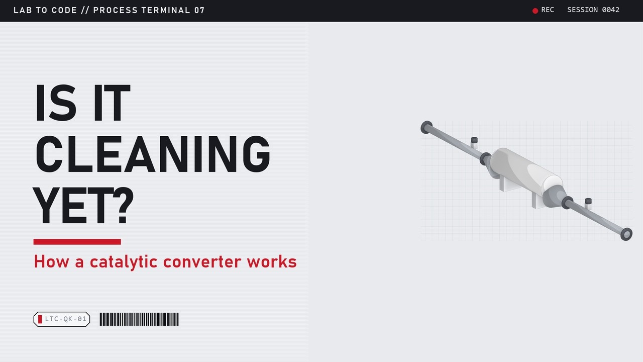
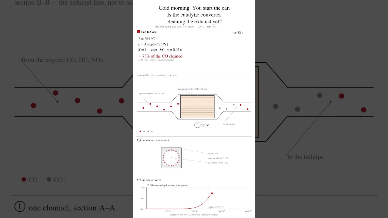
"""Lab to Code — Why a catalytic converter does nothing for the first minute: the light-off curve.

Model (illustrative parameters): CO oxidation as a first-order reaction in a plug-flow monolith,
conversion X = 1 - exp(-k * tau), with Arrhenius k = A * exp(-Ea / (R * T)).
Ea = 100 kJ/mol and A = 3.4e11 1/s are chosen so that 50 % conversion ("light-off") lands near 250 C,
inside the typical range for real converters (a few hundred C). tau = 0.02 s is the gas residence time.
"""
from math import exp

R, EA, A, TAU = 8.314, 100e3, 3.4e11, 0.02

for t_c in (150, 200, 250, 300, 400):
    k = A * exp(-EA / (R * (t_c + 273.15)))
    x = 1 - exp(-k * TAU)
    print(f"{t_c:3} C: k = {k:9.2f} 1/s, CO converted {x:6.1%}")
SALIDA REALREAL OUTPUT
150 C: k =      0.15 1/s, CO converted   0.3%
200 C: k =      3.10 1/s, CO converted   6.0%
250 C: k =     35.19 1/s, CO converted  50.5%
300 C: k =    261.54 1/s, CO converted  99.5%
400 C: k = 5908.35 1/s, CO converted 100.0%CODEDESCARGAR .PYDOWNLOAD .PY · VER EL VIDEOWATCH THE VIDEO →
"""Lab to Code — Why a catalytic converter does nothing for the first minute: the light-off curve.

Model (illustrative parameters): CO oxidation as a first-order reaction in a plug-flow monolith,
conversion X = 1 - exp(-k * tau), with Arrhenius k = A * exp(-Ea / (R * T)).
Ea = 100 kJ/mol and A = 3.4e11 1/s are chosen so that 50 % conversion ("light-off") lands near 250 C,
inside the typical range for real converters (a few hundred C). tau = 0.02 s is the gas residence time.
"""
from math import exp

R, EA, A, TAU = 8.314, 100e3, 3.4e11, 0.02

for t_c in (150, 200, 250, 300, 400):
    k = A * exp(-EA / (R * (t_c + 273.15)))
    x = 1 - exp(-k * TAU)
    print(f"{t_c:3} C: k = {k:9.2f} 1/s, CO converted {x:6.1%}")
SALIDA REALREAL OUTPUT
150 C: k =      0.15 1/s, CO converted   0.3%
200 C: k =      3.10 1/s, CO converted   6.0%
250 C: k =     35.19 1/s, CO converted  50.5%
300 C: k =    261.54 1/s, CO converted  99.5%
400 C: k = 5908.35 1/s, CO converted 100.0%CODEDESCARGAR .PYDOWNLOAD .PY · VER EL VIDEOWATCH THE VIDEO →
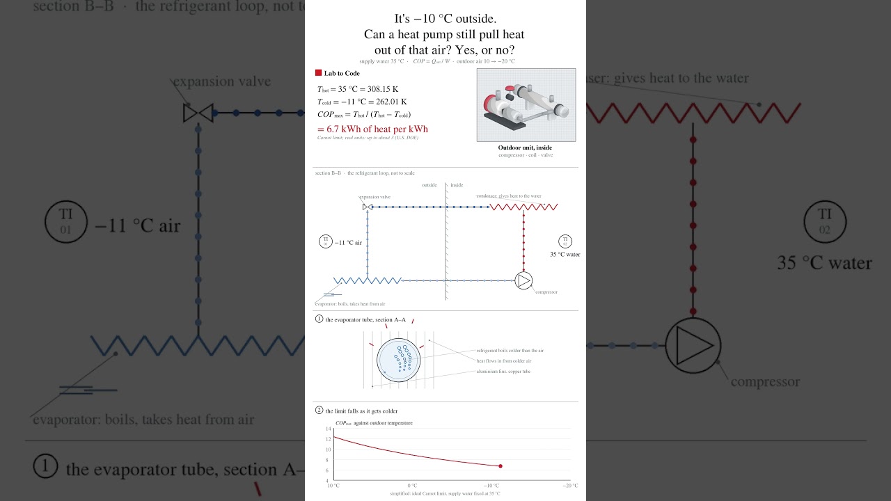
"""Lab to Code — How much heat can a heat pump move per kWh? The Carnot limit.

The best possible coefficient of performance for heating is COP = T_hot / (T_hot - T_cold), temperatures in kelvin
(second law of thermodynamics; any textbook, e.g. Cengel and Boles, Thermodynamics). Real units deliver less:
up to about 3 kWh of heat per kWh of electricity in moderate climates (U.S. DOE, Solar Decathlon).
T_hot is the water you send to the house: about 35 C for floor heating, about 55 C for old radiators.
"""
SUPPLY = {"floor heating": 35, "radiators": 55}   # C

for t_out in (10, 0, -10, -20):
    cops = []
    for name, t_in in SUPPLY.items():
        th, tc = t_in + 273.15, t_out + 273.15
        cops.append(f"{name} {th / (th - tc):.1f}")
    print(f"{t_out:4} C outside: Carnot COP " + ", ".join(cops))
SALIDA REALREAL OUTPUT
  10 C outside: Carnot COP floor heating 12.3, radiators 7.3
   0 C outside: Carnot COP floor heating 8.8, radiators 6.0
 -10 C outside: Carnot COP floor heating 6.8, radiators 5.0
-20 C outside: Carnot COP floor heating 5.6, radiators 4.4CODEDESCARGAR .PYDOWNLOAD .PY · VER EL VIDEOWATCH THE VIDEO →
"""Lab to Code — How much heat can a heat pump move per kWh? The Carnot limit.

The best possible coefficient of performance for heating is COP = T_hot / (T_hot - T_cold), temperatures in kelvin
(second law of thermodynamics; any textbook, e.g. Cengel and Boles, Thermodynamics). Real units deliver less:
up to about 3 kWh of heat per kWh of electricity in moderate climates (U.S. DOE, Solar Decathlon).
T_hot is the water you send to the house: about 35 C for floor heating, about 55 C for old radiators.
"""
SUPPLY = {"floor heating": 35, "radiators": 55}   # C

for t_out in (10, 0, -10, -20):
    cops = []
    for name, t_in in SUPPLY.items():
        th, tc = t_in + 273.15, t_out + 273.15
        cops.append(f"{name} {th / (th - tc):.1f}")
    print(f"{t_out:4} C outside: Carnot COP " + ", ".join(cops))
SALIDA REALREAL OUTPUT
  10 C outside: Carnot COP floor heating 12.3, radiators 7.3
   0 C outside: Carnot COP floor heating 8.8, radiators 6.0
 -10 C outside: Carnot COP floor heating 6.8, radiators 5.0
-20 C outside: Carnot COP floor heating 5.6, radiators 4.4CODEDESCARGAR .PYDOWNLOAD .PY · VER EL VIDEOWATCH THE VIDEO →
"""Lab to Code — Why the grid runs at high voltage, and how much CO2 one kWh costs.

1) Line loss: the same power P = V * I at a higher voltage needs less current, and the loss is I^2 * R.
   Simplified: one conductor, 100 km at about 0.05 ohm/km, single-phase equivalent (real lines are 3-phase).
2) CO2 per kWh: heat of combustion (NIST: CH4 -890.3 kJ/mol, C -393.5 kJ/mol) and the plant heat rate
   (EIA 2025 average operating heat rates: natural gas 7,781 Btu/kWh, coal 10,647 Btu/kWh; 1 kWh = 3,412 Btu).
   Coal is treated as pure carbon, so its number is an upper bound.
"""
P = 100e6          # W sent down the line (100 MW)
R = 5.0            # ohm: 100 km x 0.05 ohm/km

for kv in (13.8, 138, 345):
    I = P / (kv * 1e3)                    # amps needed
    loss = I ** 2 * R                     # watts turned into heat
    print(f"{kv:5} kV: {I:5.0f} A, loss {100 * loss / P:6.1f}%")

FUEL = {"gas": (890.3, 7781),             # kJ/mol released, Btu per kWh
        "coal": (393.5, 10647)}
for name, (dH, heat_rate) in FUEL.items():
    eff = 3412 / heat_rate                # plant efficiency
    mol = 3600 / (dH * eff)               # mol of fuel per kWh (3600 kJ)
    print(f"{name}: eff {eff:.0%}, {mol * 44.01:.0f} g CO2/kWh")
SALIDA REALREAL OUTPUT
 13.8 kV:  7246 A, loss  262.5%
  138 kV:   725 A, loss    2.6%
  345 kV:   290 A, loss    0.4%
gas: eff 44%, 406 g CO2/kWh
coal: eff 32%, 1256 g CO2/kWhCODEDESCARGAR .PYDOWNLOAD .PY · VER EL VIDEOWATCH THE VIDEO →
"""Lab to Code — How many trays does a distillation column need? (benzene + toluene, Fenske equation)

Relative volatility: alpha = Psat_benzene / Psat_toluene (Raoult's law, ideal mixture). Psat from the Antoine
equation (NIST WebBook, P in bar, T in K): log10(Psat) = A - B / (T + C), the same constants as our Raoult video.
Fenske: minimum number of stages at total reflux
    N_min = ln[(xD / (1 - xD)) * ((1 - xB) / xB)] / ln(alpha)
"""
from math import log, sqrt

ANT = {"benzene": (4.01814, 1203.835, -53.226), "toluene": (4.07827, 1343.943, -53.773)}
P = 1.01325  # bar


def psat(name, T):
    A, B, C = ANT[name]
    return 10 ** (A - B / (T + C))


def boiling_T(x, lo=340.0, hi=390.0):        # bisection, as in the Raoult video
    for _ in range(50):
        mid = (lo + hi) / 2
        total = x * psat("benzene", mid) + (1 - x) * psat("toluene", mid)
        lo, hi = (lo, mid) if total == max(total, P) else (mid, hi)
    return mid


def fenske(xD, xB, a):
    return log((xD / (1 - xD)) * ((1 - xB) / xB)) / log(a)


Tt, Tb = boiling_T(0.95), boiling_T(0.05)
a = sqrt(psat("benzene", Tt) / psat("toluene", Tt) * psat("benzene", Tb) / psat("toluene", Tb))
print(f"top {Tt - 273.15:.1f} C, bottom {Tb - 273.15:.1f} C, alpha {a:.2f}")
for xD in (0.95, 0.99):
    print(f"{xD:.0%} pure: {fenske(xD, 1 - xD, a):.1f} stages min")
SALIDA REALREAL OUTPUT
top 81.1 C, bottom 108.3 C, alpha 2.47
95% pure: 6.5 stages min
99% pure: 10.1 stages minCODEDESCARGAR .PYDOWNLOAD .PY · VER EL VIDEOWATCH THE VIDEO →
"""Lab to Code — What the sensors in a refinery actually measure.

Two of the most common transmitters in a plant turn a pressure into something else:
- Level (LT): a differential-pressure transmitter reads the weight of the liquid column. h = dP / (rho * g)
- Flow (FT): an orifice plate creates a pressure drop. Q = Cd * A * sqrt(2 * dP / rho)
Typical values: crude oil density ~850 kg/m3; orifice discharge coefficient Cd ~0.61.
"""
from math import pi, sqrt

G = 9.81            # m/s^2
RHO_CRUDE = 850     # kg/m^3


def level_from_dp(dp_kpa, rho=RHO_CRUDE):
    return dp_kpa * 1000 / (rho * G)                     # meters of liquid


def flow_from_orifice(dp_kpa, d_mm, rho=RHO_CRUDE, cd=0.61):
    area = pi * (d_mm / 1000) ** 2 / 4                   # m^2
    q = cd * area * sqrt(2 * dp_kpa * 1000 / rho)        # m^3/s
    return q * 3600                                      # m^3/h


for dp in (25, 50):
    print(f"LT: {dp} kPa → {level_from_dp(dp):.1f} m of crude")
for dp in (10, 40):
    print(f"FT: {dp} kPa across a 100 mm orifice → {flow_from_orifice(dp, 100):.0f} m3/h")
SALIDA REALREAL OUTPUT
LT: 25 kPa → 3.0 m of crude
LT: 50 kPa → 6.0 m of crude
FT: 10 kPa across a 100 mm orifice → 84 m3/h
FT: 40 kPa across a 100 mm orifice → 167 m3/hCODEDESCARGAR .PYDOWNLOAD .PY · VER EL VIDEOWATCH THE VIDEO →
"""Lab to Code — 2026 Nobel Prize in Chemistry (Kagan, Soai): a toy model of non-linear autocatalysis.

Not the real Soai mechanism: a minimal model where the speed depends on the enantiomeric excess,
which is enough to amplify a tiny imbalance until only one "hand" is left.
"""
L, D = 1.001, 1.000           # two mirror forms, 0.1 % apart
K, ALPHA, DT = 0.9, 0.9, 0.01  # base speed, weight of the excess, time step


def ee(l, d):
    """Enantiomeric excess, from -1 (all D) to +1 (all L)."""
    return (l - d) / (l + d)


hist = []
for step in range(4000):
    e = ee(L, D)
    L += K * L * (1 + ALPHA * e) * DT   # the speed depends on the excess: that's the non-linear part
    D += K * D * (1 - ALPHA * e) * DT
    hist.append((step * DT, ee(L, D)))

start, final = hist[0][1], hist[-1][1]
t99 = next(t for t, e in hist if max(e, 0.99) == e)   # first time the excess reaches 99 %
print(f"start ee: {start * 100:.2f} %")
print(f"final ee: {final * 100:.2f} %")
print(f"time to 99 % ee: {t99:.1f} (model units)")
print(f"amplification: {final / start:,.0f}x")
SALIDA REALREAL OUTPUT
start ee: 0.05 %
final ee: 100.00 %
time to 99 % ee: 11.9 (model units)
amplification: 1,985xCODEDESCARGAR .PYDOWNLOAD .PY · VER EL VIDEOWATCH THE VIDEO →
"""Lab to Code — 2026 Nobel Prize in Physiology or Medicine (optogenetics): light makes a neuron fire.

A toy integrate-and-fire neuron with a light-gated conductance (not Hodgkin-Huxley, not real optogenetics).
"""
V_rest, V_th, V_reset = -70.0, -55.0, -80.0     # mV
g_leak, g_light, C, dt = 10.0, 8.0, 1.0, 0.1    # conductances, capacitance, time step (ms)

light = [0.0] * 120                             # two blue-light pulses of 1 ms
for k in list(range(20, 30)) + list(range(70, 80)):
    light[k] = 1.0

V, spikes, refractory = V_rest, [], 0
for i in range(120):
    g = g_light * light[i]
    I = -g_leak * (V - V_rest) + g * (0.0 - V)    # light adds a depolarizing conductance
    if refractory:
        V = V_reset
        refractory -= 1
    else:
        V += dt * I / C
        if V == max(V, V_th):                     # same as "V at or above the threshold"
            spikes.append(round(i * dt, 1))
            V = V_reset
            refractory = 3

print("light pulses: 2.0-2.9 ms and 7.0-7.9 ms")
print(f"spikes: {len(spikes)} at {spikes} ms")
SALIDA REALREAL OUTPUT
light pulses: 2.0-2.9 ms and 7.0-7.9 ms
spikes: 6 at [2.0, 2.4, 2.8, 7.0, 7.4, 7.8] msCODEDESCARGAR .PYDOWNLOAD .PY · VER EL VIDEOWATCH THE VIDEO →
"""Lab to Code — 2026 Nobel Prize in Physics (IceCube): the Cherenkov cone in ice.

A charged particle moving faster than light does in ice emits light in a cone: cos(theta) = 1 / (n * beta).
"""
from math import acos, degrees

C = 299_792_458.0      # speed of light in vacuum, m/s
N_ICE = 1.31           # refractive index of glacial ice


def cherenkov_deg(n, beta=1.0):
    """Angle of the Cherenkov cone, in degrees."""
    return degrees(acos(1.0 / (n * beta)))


v = C / N_ICE
print(f"Cherenkov cone in ice: {cherenkov_deg(N_ICE):.1f} deg")
print(f"light speed in ice: {v / 1e6:.1f} km/ms")
print(f"time to cross 100 m: {100.0 / v * 1e9:.0f} ns")
SALIDA REALREAL OUTPUT
Cherenkov cone in ice: 40.2 deg
light speed in ice: 228.8 km/ms
time to cross 100 m: 437 nsCODEDESCARGAR .PYDOWNLOAD .PY · VER EL VIDEOWATCH THE VIDEO →
"""Lab to Code — Bread from air: how pressure pushes the Haber-Bosch equilibrium (ideal-gas estimate).

N2 + 3 H2 <-> 2 NH3, fed 1 : 3. Kp = 1.45e-5 atm^-2 at 500 C (textbook value).
"""
KP_500C = 1.45e-5   # atm^-2


def ammonia_share(P, Kp=KP_500C):
    """Mole fraction of NH3 at equilibrium, total pressure P in atm (bisection on the extent)."""
    def gap(z):                       # z = mol of N2 that reacted, starting from 1 N2 + 3 H2
        n = 4 - 2 * z
        y_n2, y_h2, y_nh3 = (1 - z) / n, (3 - 3 * z) / n, 2 * z / n
        return y_nh3**2 / (y_n2 * y_h2**3 * P**2) - Kp
    lo, hi = 0.0, 0.999999
    for _ in range(60):
        mid = (lo + hi) / 2
        lo, hi = (lo, mid) if gap(mid) > 0 else (mid, hi)
    z = (lo + hi) / 2
    return 2 * z / (4 - 2 * z)


for P in (1, 100, 200, 300):
    print(f"{P:>3} atm: {100 * ammonia_share(P):.1f}% ammonia")
SALIDA REALREAL OUTPUT
  1 atm: 0.1% ammonia
100 atm: 10.0% ammonia
200 atm: 17.0% ammonia
300 atm: 22.4% ammoniaCODEDESCARGAR .PYDOWNLOAD .PY · VER EL VIDEOWATCH THE VIDEO →
"""Lab to Code — How an airbag inflates: stoichiometry + the ideal gas law.

Reaction in the classic inflator: 2 NaN3 to 2 Na + 3 N2 (2 mol of sodium azide give 3 mol of nitrogen).
Molar mass of NaN3: 65.01 g/mol (PubChem). Ideal gas law: P V = n R T.
"""
M_NAN3 = 65.01      # g/mol
R = 0.08206         # L*atm/(mol*K)


def liters_of_n2(grams, T_C=25, P_atm=1.0):
    mol_azide = grams / M_NAN3
    mol_n2 = mol_azide * 3 / 2          # the 3:2 ratio from the equation
    return mol_n2 * R * (T_C + 273.15) / P_atm


def grams_for(liters, T_C=25, P_atm=1.0):
    mol_n2 = P_atm * liters / (R * (T_C + 273.15))
    return mol_n2 * 2 / 3 * M_NAN3


print(f"65 g of NaN3 gives {liters_of_n2(65):.1f} L of N2 at 25 C")
print(f"A 60 L bag needs {grams_for(60):.0f} g of NaN3")
print(f"If the gas were at 300 C: {liters_of_n2(65, 300):.1f} L")
SALIDA REALREAL OUTPUT
65 g of NaN3 gives 36.7 L of N2 at 25 C
A 60 L bag needs 106 g of NaN3
If the gas were at 300 C: 70.5 LCODEDESCARGAR .PYDOWNLOAD .PY · VER EL VIDEOWATCH THE VIDEO →
"""Lab to Code — Arrhenius: why heat speeds up reactions.

k = A * exp(-Ea / (R * T)). The ratio between two temperatures doesn't need A:
k2 / k1 = exp(Ea / R * (1/T1 - 1/T2))
"""
from math import exp

R = 8.314          # J/(mol*K)
Ea = 50_000        # J/mol, a typical activation energy


def rate_ratio(T1_C, T2_C, Ea=Ea):
    T1, T2 = T1_C + 273.15, T2_C + 273.15   # always use kelvin
    return exp(Ea / R * (1 / T1 - 1 / T2))


print(f"25 -> 35 C: {rate_ratio(25, 35):.2f}x faster")
print(f"25 -> 45 C: {rate_ratio(25, 45):.2f}x faster")
print(f"25 ->  5 C: {rate_ratio(25, 5):.2f}x (slower)")
SALIDA REALREAL OUTPUT
25 -> 35 C: 1.92x faster
25 -> 45 C: 3.55x faster
25 -> 5 C: 0.23x (slower)CODEDESCARGAR .PYDOWNLOAD .PY · VER EL VIDEOWATCH THE VIDEO →
"""Lab to Code — Is your process capable? Cp and Cpk.

Bottle fill volume, spec 500 +/- 6 mL. 50 bottles measured (simulated with a fixed seed).
Cp  = (USL - LSL) / (6 * sigma)                -> could the process fit, if it were centered?
Cpk = min(USL - mean, mean - LSL) / (3 * sigma) -> does it fit, where it actually is?
"""
import numpy as np

LSL, USL = 494.0, 506.0

rng = np.random.default_rng(7)
fills = rng.normal(loc=503.0, scale=1.2, size=50)   # off-center: mean near 503, not 500

mean = fills.mean()
sigma = fills.std(ddof=1)
cp = (USL - LSL) / (6 * sigma)
cpk = min(USL - mean, mean - LSL) / (3 * sigma)

print(f"mean = {mean:.2f} mL, sigma = {sigma:.2f} mL")
print(f"Cp  = {cp:.2f}")
print(f"Cpk = {cpk:.2f}")
print("capable" if cpk >= 1.33 else "not capable yet: center it first")
SALIDA REALREAL OUTPUT
mean = 502.65 mL, sigma = 1.07 mL
Cp  = 1.86
Cpk = 1.04
not capable yet: center it firstCODEDESCARGAR .PYDOWNLOAD .PY · VER EL VIDEOWATCH THE VIDEO →
"""Lab to Code — How an airbag inflates: stoichiometry + the ideal gas law.

Reaction in the classic inflator: 2 NaN3 to 2 Na + 3 N2 (2 mol of sodium azide give 3 mol of nitrogen).
Molar mass of NaN3: 65.01 g/mol (PubChem). Ideal gas law: P V = n R T.
"""
M_NAN3 = 65.01      # g/mol
R = 0.08206         # L*atm/(mol*K)


def liters_of_n2(grams, T_C=25, P_atm=1.0):
    mol_azide = grams / M_NAN3
    mol_n2 = mol_azide * 3 / 2          # the 3:2 ratio from the equation
    return mol_n2 * R * (T_C + 273.15) / P_atm


def grams_for(liters, T_C=25, P_atm=1.0):
    mol_n2 = P_atm * liters / (R * (T_C + 273.15))
    return mol_n2 * 2 / 3 * M_NAN3


print(f"65 g of NaN3 gives {liters_of_n2(65):.1f} L of N2 at 25 C")
print(f"A 60 L bag needs {grams_for(60):.0f} g of NaN3")
print(f"If the gas were at 300 C: {liters_of_n2(65, 300):.1f} L")
SALIDA REALREAL OUTPUT
65 g of NaN3 gives 36.7 L of N2 at 25 C
A 60 L bag needs 106 g of NaN3
If the gas were at 300 C: 70.5 LCODEDESCARGAR .PYDOWNLOAD .PY · VER EL VIDEOWATCH THE VIDEO →
"""Lab to Code — Is your process out of control? An individuals control chart.

Same bottle filler as the Cp/Cpk video: target 500 mL. 30 bottles in a row (simulated with a fixed seed).
The first 20 set the limits; after bottle 20 the machine drifts up by 2 mL.
Limits for an individuals chart: center = mean, UCL/LCL = mean +/- 2.66 * average moving range.
"""
import numpy as np

rng = np.random.default_rng(3)
fills = np.round(np.concatenate([rng.normal(500.0, 1.0, 20),
                                 rng.normal(502.0, 1.0, 10)]), 1)

base = fills[:20]                        # limits come from the stable period
center = base.mean()
mr_bar = np.abs(np.diff(base)).mean()    # average moving range
ucl = center + 2.66 * mr_bar
lcl = center - 2.66 * mr_bar
print(f"center = {center:.2f}  UCL = {ucl:.2f}  LCL = {lcl:.2f}")

# Rule 1: a point outside the limits
out = [i + 1 for i, x in enumerate(fills) if max(x, ucl) != ucl or min(x, lcl) != lcl]
print("outside the limits:", out)

# Rule 2: eight points in a row on the same side of the center line
side = np.sign(fills - center)
for i in range(len(fills) - 7):
    if abs(side[i:i + 8].sum()) == 8:
        print("8 in a row on one side, ending at bottle", i + 8)
        break
SALIDA REALREAL OUTPUT
center = 499.85  UCL = 503.61  LCL = 496.10
outside the limits: [27]
8 in a row on one side, ending at bottle 28CODEDESCARGAR .PYDOWNLOAD .PY · VER EL VIDEOWATCH THE VIDEO →
"""Lab to Code — Is your process capable? Cp and Cpk.

Bottle fill volume, spec 500 +/- 6 mL. 50 bottles measured (simulated with a fixed seed).
Cp  = (USL - LSL) / (6 * sigma)                -> could the process fit, if it were centered?
Cpk = min(USL - mean, mean - LSL) / (3 * sigma) -> does it fit, where it actually is?
"""
import numpy as np

LSL, USL = 494.0, 506.0

rng = np.random.default_rng(7)
fills = rng.normal(loc=503.0, scale=1.2, size=50)   # off-center: mean near 503, not 500

mean = fills.mean()
sigma = fills.std(ddof=1)
cp = (USL - LSL) / (6 * sigma)
cpk = min(USL - mean, mean - LSL) / (3 * sigma)

print(f"mean = {mean:.2f} mL, sigma = {sigma:.2f} mL")
print(f"Cp  = {cp:.2f}")
print(f"Cpk = {cpk:.2f}")
print("capable" if cpk >= 1.33 else "not capable yet: center it first")
SALIDA REALREAL OUTPUT
mean = 502.65 mL, sigma = 1.07 mL
Cp  = 1.86
Cpk = 1.04
not capable yet: center it firstCODEDESCARGAR .PYDOWNLOAD .PY · VER EL VIDEOWATCH THE VIDEO →
"""Lab to Code — Arrhenius: why heat speeds up reactions.

k = A * exp(-Ea / (R * T)). The ratio between two temperatures doesn't need A:
k2 / k1 = exp(Ea / R * (1/T1 - 1/T2))
"""
from math import exp

R = 8.314          # J/(mol*K)
Ea = 50_000        # J/mol, a typical activation energy


def rate_ratio(T1_C, T2_C, Ea=Ea):
    T1, T2 = T1_C + 273.15, T2_C + 273.15   # always use kelvin
    return exp(Ea / R * (1 / T1 - 1 / T2))


print(f"25 -> 35 C: {rate_ratio(25, 35):.2f}x faster")
print(f"25 -> 45 C: {rate_ratio(25, 45):.2f}x faster")
print(f"25 ->  5 C: {rate_ratio(25, 5):.2f}x (slower)")
SALIDA REALREAL OUTPUT
25 -> 35 C: 1.92x faster
25 -> 45 C: 3.55x faster
25 -> 5 C: 0.23x (slower)CODEDESCARGAR .PYDOWNLOAD .PY · VER EL VIDEOWATCH THE VIDEO →
"""Lab to Code — Where does equilibrium land? Solve it with bisection.

A + B <=> C, K = 4, start with [A] = [B] = 1 M and no C.
Let x = mol/L of C formed. At equilibrium: x / (1 - x)**2 = K.
Rewrite as f(x) = x - K * (1 - x)**2 = 0 and find the root between 0 and 1.
"""


def f(x, K=4):
    return x - K * (1 - x) ** 2


def bisection(f, low, high, tol=1e-6):
    steps = 0
    while high - low > tol:
        mid = (low + high) / 2
        if f(low) * f(mid) <= 0:   # sign change on the left half
            high = mid
        else:                      # otherwise it's in the right half
            low = mid
        steps += 1
    return (low + high) / 2, steps


x, steps = bisection(f, 0, 1)
print(f"x = {x:.4f} M ({steps} steps)")
print(f"[A] = [B] = {1 - x:.3f} M, [C] = {x:.3f} M")
print(f"check K: {x / (1 - x) ** 2:.3f}")
SALIDA REALREAL OUTPUT
x = 0.6096 M (20 steps)
[A] = [B] = 0.390 M, [C] = 0.610 M
check K: 4.000CODEDESCARGAR .PYDOWNLOAD .PY · VER EL VIDEOWATCH THE VIDEO →
"""Lab to Code — Q vs K: which way will the reaction go?

Reaction quotient: Q = product of (concentration ** coefficient) over all species,
with negative coefficients for reactants. Compare Q with K to get the direction.
"""
from math import isclose


def reaction_quotient(conc, coeffs):
    q = 1.0
    for species, nu in coeffs.items():  # nu > 0: product, nu < 0: reactant
        q *= conc[species] ** nu
    return q


def direction(Q, K):
    if isclose(Q, K):
        return "equilibrium"
    return "forward" if Q < K else "reverse"


# A + B <=> C   with K = 4
coeffs = {"A": -1, "B": -1, "C": 1}
conc = {"A": 1.0, "B": 1.0, "C": 2.0}  # mol/L, right now

Q = reaction_quotient(conc, coeffs)
print(f"Q = {Q}")
print(direction(Q, K=4))
SALIDA REALREAL OUTPUT
Q = 2.0
forward
Cada script se ejecutó con Python 3.11.15 el 2026-11-05 y la salida es la que imprimió.Every script was run with Python 3.11.15 on 2026-11-05; the output is what it printed.